Analog and digital
Digital does not mean electronic but finitely many clearly separated states. That is why a small disturbance changes a value but not a state, and getting there takes two cuts whose price you can count in bytes and minutes.
What you will learn
Using a link that sends data with light, this lesson explains what digital really means and what it costs to get there, and afterwards you can:
- define digital as finitely many clearly separated states and sort everyday things such as a dimmer, a die or a split-flap display into analog and digital
- explain why a small disturbance changes an analog value but not a digital state, and why digital copies therefore do not inherit the noise
- explain why the same scatter of readings that two regions absorb easily pushes readings into the neighbouring region when there are eight
- tell sampling from quantising and recognise from blocks or hard patches which of the two cuts was too coarse
- estimate the size of a picture as points times bits per point and turn it into a transmission time
- set a threshold in code that turns a reading into a symbol and justify its value from your own measurement series
Picture the departures board of a railway station before the age of chips: the split-flap display clatters until every letter has fallen into place. There is no computer anywhere near it, and yet the board is perfectly digital, because every flap rests in exactly one of its positions and while it turns there is no valid state in between. That is also why you can read it from twenty metres away, and it shows the point of this lesson from the start: digital is a question of states, not of electronics.
Finitely many states, and nothing in between
The scoreboard in a sports hall that you flip by hand is digital, and so are the light switch, the abacus and the die. The slide rule, the dial thermometer, the dimmer and the hourglass are analog. Not one of these things contains a chip, so digital cannot mean electronic. The reverse holds as well: an amplifier is electronic and still stepless, so electronics is only today's usual carrier of digital states.
An analog quantity can take any value at all: between any two values lies another one, and there is no smallest step. A digital system works the other way round, and its definition mentions no electricity at all: digital means finitely many states, and nothing in between counts.
The second half of that sentence is the important one. A reading that lies somewhere between the states is simply assigned to the nearest state, and so a small disturbance has no effect.
The same disturbance, twice
What that looks like shows the same disturbance in two worlds. Each has two upright scales from 0 to 400, the sender's on the left and the receiver's on the right, so that the way runs to the right and the value runs up. The sender sends 300, and 23 are added on the way, so 323 arrives at the receiver, the yellow dot; the dashed line shows where 300 would have been.
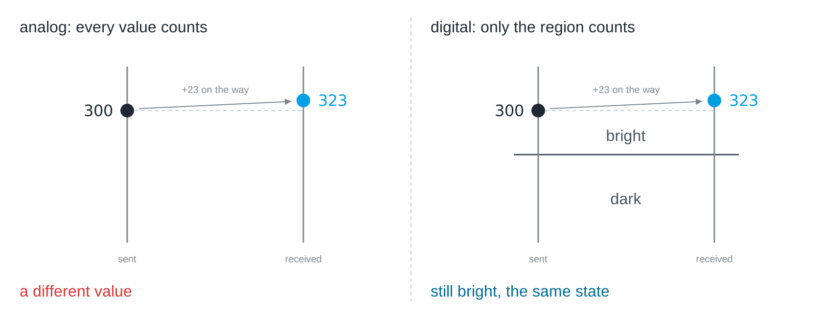
In an analog signal every value counts, so the received one is simply a different value, and the disturbance has become part of the signal. In a digital signal only the region counts: a boundary at 200 divides both scales into dark and bright, 323 lies in the bright region just like 300 and therefore means the same state. Try it:
sent = 300          # the value the sender means
disturbance = 23    # what the way through the room adds
received = sent + disturbance

threshold = 200     # the boundary between dark and bright

def state(value):
    if value > threshold:
        return "bright"
    return "dark"

print("analog:  sent", sent, "- received", received)
print("digital: sent", state(sent), "- received", state(received))
Analog, a different value arrives; digital, the same state. Set the
disturbance to -120, and the digital state flips as well, because now the
disturbance is larger than the distance to the boundary. Digital does not
make disturbances impossible; it only makes every disturbance harmless that
is smaller than this distance.
The part no program controls
Take a link that sends data with light. A program sets the brightness of an
LED with numbers, for example (255, 0, 0) for full red, the light crosses the
room, and a colour sensor at the other end turns it back into numbers. The
link therefore runs through three zones, digital, analog and digital again.
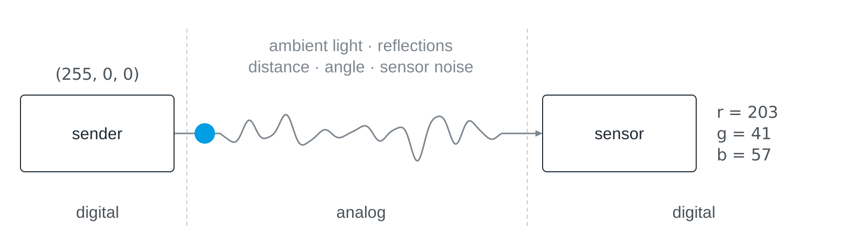
The middle is physics, and many things disturb it: ambient light from the windows and the ceiling lamps, reflections from the table and from clothes, the distance and the angle between LED and sensor, and the noise of the sensor itself, which never measures exactly the same value twice. No program has any say in this. Whoever forgets this analog middle will later be surprised by every disturbance, and whoever takes it seriously knows why you have to measure.
Light has no steps, but your program needs them
The light itself is analog, since between any two brightnesses lies another. What the program at the receiving end needs is the opposite, a few states that are clearly apart.
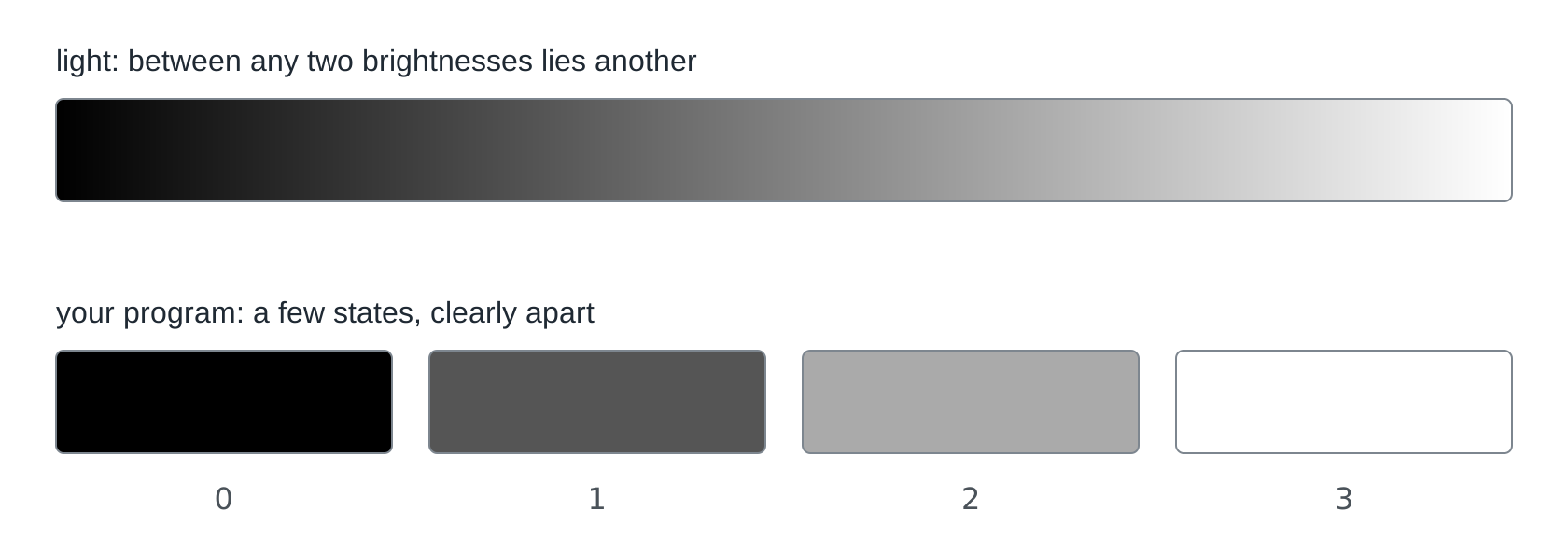
The program gets these states in two steps: the sensor measures and delivers a number, and the program decides which state that number belongs to. That is all the word digitising means: representing a signal by a finite sequence of numbers.
The same scatter, cut into more regions
Two states are safe, but they carry little per reading. Four or eight states would carry more, and how many you can afford has a picture, the one to remember from this lesson.
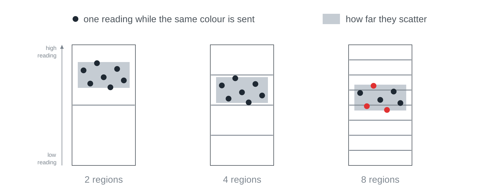
The vertical axis is what the sensor reports, for example the reading of the clear channel. Each of the three columns is the same range of readings, cut into two, four and eight regions, so for an alphabet of two, four or eight colours. Each dot is one reading while the sender keeps showing the same colour, and because the disturbances of the middle never rest, the readings never agree exactly. The grey band shows how far they scatter, and it is equally wide in all three columns, because the light link is the same.
From left to right the scatter did not grow; the margin shrank. The distance from the middle of a region to the next boundary is your safety reserve, and more regions spread the same reserve over more boundaries. The program checks the same with numbers, using the same seven deviations as the drawing:
low, high = 0, 420         # the range of readings
levels = 2                 # try 4 and 8

# how far seven readings of the same colour lay from the value that was sent
scatter = [-16, 30, -41, 8, 43, -21, 19]

width = (high - low) / levels
target = levels // 2       # the region just above the middle
sent = low + (target + 0.5) * width

regions = []
for s in scatter:
    regions.append(int((sent + s - low) // width))

print("Each region is", width, "wide")
print("From the middle to the boundary:", width / 2, "- largest deviation:", max(abs(s) for s in scatter))
print("Regions read:", regions)
print("In the wrong region:", len(regions) - regions.count(target), "of", len(regions))
With two regions the boundary lies 105 away from the middle, the largest deviation is 43, and all seven readings land in the right region. With four regions the distance shrinks to 52.5, which is still enough but no longer generous. With eight it is only 26.25, and three of the seven readings land in a neighbouring region. The scatter was the same each time; only the boundaries came closer.
Eight regions would be worth having, because each reading would then carry three bits instead of one, as Symbols and information explains. This is the same argument that explains why computers work with two states, here applied to a sensor instead of a wire. The other half of the problem is in Signal and noise: there the number of symbols stays put and the spread of the readings is measured instead, and both roads end at the same wall.
What the thrown-away precision buys
Digitising is a one-way street. Once a reading has been assigned to a region, nobody can tell any more which of the infinitely many values inside that region it really was. That loss is not an accident but the price, and two chains of copies show what it buys.
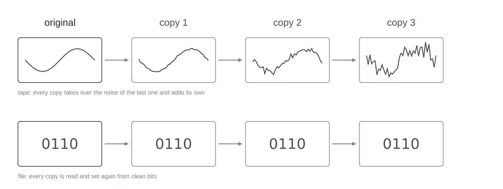
Above, a tape: each copy records the wave of the previous copy, together with
all the noise already in it, and adds noise of its own. The noise therefore
piles up, and the wave gets rougher from copy to copy. Below, a file: at
every copy the bits are read, 0110 is recognised, and the copy is set again
from these clean bits, so 0110 stays 0110. The program copies both ten
times in a row:
import random

random.seed(4)
noise = 0.1                   # how much every copy adds, at most

tape = [0.0, 1.0, 1.0, 0.0]   # the original as a stepless signal
file = [0, 1, 1, 0]           # the original as bits

for copy in range(10):
    # the tape keeps whatever arrives, noise included
    tape = [v + random.uniform(-noise, noise) for v in tape]
    # the file is read again: above the middle counts as 1, below as 0
    file = [1 if v + random.uniform(-noise, noise) > 0.5 else 0 for v in file]

print("Tape after 10 copies:", [round(v, 2) for v in tape])
print("File after 10 copies:", file)
After ten copies the tape has drifted away from the original, while the file
is still exactly [0, 1, 1, 0]. Set noise to 0.6, and the file flips as
well, because then a single disturbance is larger than half the distance
between 0 and 1.
Every disturbance smaller than that distance disappears completely when the state is read, and that is why the thousandth copy of a file is still the original. Digital technology is reliable not although it throws information away but because it does.
Two cuts
Digitising a picture takes two cuts. The first cut goes through the area: the stepless picture becomes measuring points, for example 16 × 16. That is sampling, and how fine it is, is the resolution. The second cut goes through the value: the brightness of every point is rounded to one of the agreed levels, for example four grey levels. That is quantising, and the number of levels is the colour depth. Those levels are exactly the regions from the section above, now applied to a picture.
Both cuts throw detail away, but they leave different traces, which is how you tell which knob to turn. A picture made of visible blocks had too few points, so the sampling was too coarse. A picture whose soft shading breaks into hard patches or stripes had too few levels, so the quantising was too coarse. You can turn both knobs yourself in the Photo digitiser.
What a picture costs
One piece of arithmetic carries every file size: points × bits per point. A level needs as many bits as it takes to tell all levels apart, so four grey levels need two bits and 256 levels need eight, the same kⁿ as in Place value systems. The program works out what a picture of 64 × 64 points costs over a slow link that carries 30 bits per second:
points = 64 * 64
rate = 30   # bits per second

for bits_per_point in [24, 8, 2, 1]:
    size = points * bits_per_point
    minutes = size / rate / 60
    print(bits_per_point, "bit per point:", size // 8, "bytes,", round(minutes, 1), "minutes")
In full colour, with 24 bits per point, the picture takes 12,288 bytes and almost 55 minutes; in black and white, with one bit per point, it takes 512 bytes and little more than two minutes. Resolution and colour depth are therefore not fine details but the two levers the transmission time depends on: what you keep, you pay for in minutes.
How far can you go?
Make a photo ever coarser, with 128, 32, 8 and finally 2 points per edge, and somewhere in between it stops showing what it showed. People will disagree about where exactly that happens, and that disagreement is the point: there is no correct amount, only a trade-off against the transmission time that someone has to make on purpose. Whoever wants to send a picture over a light link faces exactly this question, and the photo digitiser here lets you answer it for yourself.
The same two cuts for sound
The two cuts are not a picture topic but the method, and for sound you can see them on a single curve.
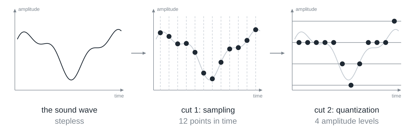
For sound, sampling slices time instead of area, and how often per second it measures is the sampling rate. Quantising slices the amplitude instead of brightness, that is how far the air is pushed out of place, which the microphone turns into a voltage; how finely it sets the levels is called the bit depth here. A CD stores 44,100 samples per second with 16 bits each. The program does to the wave of the drawing what its right-hand panel shows:
import math

samples = 12      # cut 1: how many points in time
levels = 4        # cut 2: how many amplitude levels

for i in range(samples):
    t = (i + 0.5) / samples
    value = 0.5 + 0.3 * math.sin(2 * math.pi * t * 1.3 + 0.4) + 0.12 * math.sin(2 * math.pi * t * 3.1 + 1)
    level = round(value * (levels - 1))
    print("time", round(t, 2), "- value", round(value, 3), "- level", level)
Set levels to 2, and only loud and quiet remain of the wave; set
samples to 4, and almost nothing remains of its course. The
audio digitiser here lets you hear what that sounds like: turn the sampling
rate of a recording down, and a voice soon sounds tinny.
Where your alphabet is born
The simplest decision has two states. A program that reads brightness values compares each of them with a threshold, and everything above it counts as bright, everything else as dark:
readings = [412, 398, 87, 405, 92, 79, 401, 388, 95, 410]
threshold = 250

symbols = []
for value in readings:
    if value > threshold:
        symbols.append("bright")
    else:
        symbols.append("dark")

print(symbols)
At this one comparison, hundreds of possible readings turn into two symbols. The threshold is not a constant of nature but a decision, and from here on the decision counts, not the physics. Set it to 400 and run the program again: the readings 398 and 388, which clearly belong to bright, suddenly count as dark. Where a threshold belongs is therefore not a matter of feel but of a measurement series: first measure what bright and dark really deliver, then put the threshold between them (Measuring and experimenting).
With more colours the same holds for every boundary. Two colours are safe, and eight are fast, and somewhere in between sits your alphabet. Only your own measurements know where exactly, because the width of a region has to match the scatter of the readings, and how far they scatter is known only to whoever has measured it.
Takeaways
- Digital means finitely many clearly separated states with nothing valid in between; electronics is only the usual carrier.
- A small disturbance changes an analog value but not a digital state, as long as it is smaller than the distance to the next boundary.
- Between sender and sensor, every link is analog; only a measurement and a decision make it digital again.
- More regions carry more per reading but bring the boundaries closer to the same scatter, so two regions are safe and eight may already be too many.
- Precision thrown away is the price of robustness: digital copies are reborn at every reading and do not inherit the noise.
- Digitising takes two cuts, sampling (resolution or sampling rate) and quantising (colour or bit depth), and a picture costs points × bits per point.
- A threshold or a set of regions is a decision, and it belongs where a measurement series puts it.
Builds on this
Details
- Level
- Beginner
- Modules
- Digitization and Programming
- Code
9684- Updated
- 4 November 2026
- Status
- published